HNSW vs IVFFlat in pgvector: when you really need an index

HNSW vs IVFFlat in pgvector: When You Really Need an Index

We have 10,852 vectors in production in a single table vector_store — and we're still not using either HNSW or IVFFlat. This is not an oversight. Spoiler: for most blogs and small RAG projects, an index is not needed at all until tens of thousands of rows — and when it is needed, the wrong choice between HNSW and IVFFlat can quietly break search accuracy for weeks before you notice.

Article Contents:

• 📌 What is ANN search and why brute-force isn't always bad
• 📌 How HNSW works
• 📌 How IVFFlat works
• 📌 HNSW vs IVFFlat: comparison table with numbers
• 📌 The IVFFlat trap: stale centroids
• 💼 Case 1: a blog with 800 articles — why we don't use any index
• 💼 Case 2: a service with tens of thousands of documents — why IVFFlat is appropriate there
• 💼 Practical recommendation: how to monitor the transition point
• ❓ Frequently Asked Questions (FAQ)
• ✅ Conclusions

What is ANN search and why brute-force isn't always bad

When you search for the nearest vectors to a query in pgvector, there are two paths. The first is to compare the query with every row in the table (exact nearest neighbor search). The second is to use an index that approximately finds the nearest neighbors without checking all rows (Approximate Nearest Neighbor, ANN).

The brute-force approach (no index, index-type=none in Spring AI) scales linearly — O(n). At 10,000 rows, this is milliseconds. At 10 million, it's already seconds per query, which is unacceptable for any production with traffic.

pgvector supports two main types of ANN indexes — HNSW and IVFFlat — and since version 0.8.2 (February 2026), there's also the DiskANN extension through a separate pgvectorscale package for very large datasets that exceed shared_buffers (dbi-services, March 2026). This article focuses on HNSW and IVFFlat, as these are what 95% of projects encounter.

How HNSW works

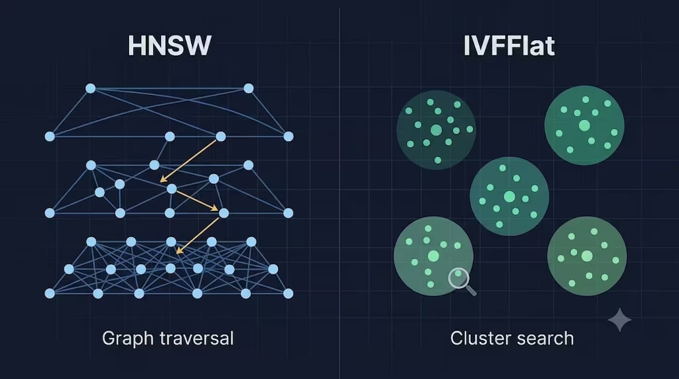
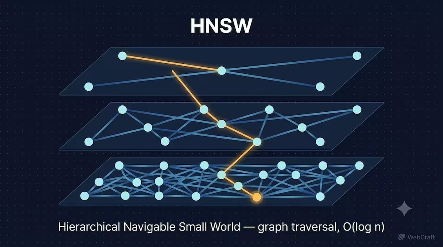
HNSW (Hierarchical Navigable Small World) builds a multi-level graph of connections between vectors. The upper levels of the graph contain sparse "expressway" connections for fast long-distance traversal, while the lower levels have dense local connections for precise final search. A query enters at the top level and "descends," narrowing the search to the nearest neighbors.

An analogy that well explains the essence: imagine searching for an address in an unfamiliar city. Instead of going down every street one by one (which is brute-force), you first get onto a highway (the upper level of the graph — long-distance "expressway" connections), drive to the desired district, and then switch to local streets (the lower level — dense local connections) to find the exact address. Each "layer" of the graph narrows the search space, hence the logarithmic complexity.

Thanks to this structure, search time grows logarithmically — O(log n) — and is independent of the order in which data was loaded (Philip McClarence, Medium, April 2026). HNSW can be built even on an empty table — the index adapts as new vectors are inserted.

Example of index creation:

CREATE INDEX ON vector_store
USING hnsw (embedding vector_cosine_ops)
WITH (m = 16, ef_construction = 64);

Here, m is the maximum number of connections per graph node (more connections = higher recall, but more memory), and ef_construction is how widely the algorithm "looks around" during index construction, searching for candidates for connections. During the search phase, there's a symmetrical parameter ef_search — it controls how many candidates are considered during the query itself:

SET hnsw.ef_search = 40;

SELECT id, content
FROM vector_store
ORDER BY embedding <=> '[0.012, -0.034, ...]'
LIMIT 10;

The default values (m=16, ef_construction=64, ef_search=40) are not random numbers but a carefully chosen starting point. Most complaints like "pgvector is slow" arise precisely because these parameters are never adjusted for a specific dataset (Nerd Level Tech, May 2026).

The price for search quality is memory and build time. An empirical rule for estimating memory usage during index construction is: N × D × 4 bytes × 2 (the multiplier 2 accounts for graph overhead) (DEV Community, March 2026). For 5 million vectors with 1536 dimensions, this means 8-16 GB of RAM just for the build process.

A ready index also takes up a lot of space: an approximate rule is 6-8 GB of RAM per million vectors with 1536 dimensions for in-memory HNSW (Groovyweb, 2026). It's worth noting: the vector dimension (1536 vs, for example, 3072) directly affects this figure — we discussed in more detail when a higher embedding dimension is truly justified in the article "1536 vs 3072: Comparing Embeddings for Document Search and RAG".

Real Memory Figures: Why HNSW "Eats" More Than It Seems

Many see the figure "6-8 GB per 1M vectors" and think that's the cost of HNSW. In reality, it's the sum of two separate components, and the second is the main drawback of HNSW, which is easily underestimated.

Example: 1 million vectors × 1536 dimensions

Here's the main drawback that's often overlooked: these 6 GB for the vectors themselves are needed in any case — even with index-type=none, even with IVFFlat. This is the base cost of data storage. The additional 1-3 GB is the pure overhead of the HNSW graph structure: an array of connections (neighbors) for each node at each graph level, which needs to be kept in memory for fast traversal.

In practice, this means: if your Postgres instance barely fits the data itself (that base 6 GB), adding an HNSW index can push the total memory consumption beyond the available shared_buffers, and part of the graph will start being pushed to disk — and this is precisely the scenario where search becomes slower, not faster, contrary to the theoretical advantage of O(log n) (dbi-services, March 2026).

IVFFlat is more honest in this regard: it doesn't add a separate connection structure on top of the data, but only stores the cluster number for each vector — hence it consumes significantly less memory beyond the base 6 GB.

A practical consequence of the maintenance_work_mem parameter: if its value is too low (Postgres default is usually 64 MB), building an HNSW index "overflows" to disk and takes 10-50 times longer (DEV Community, March 2026). Before building an index on a large dataset, it's worth temporarily increasing this parameter:

SET maintenance_work_mem = '2GB';

CREATE INDEX ON vector_store
USING hnsw (embedding vector_cosine_ops);

-- after building, you can reset to default
RESET maintenance_work_mem;

How IVFFlat works

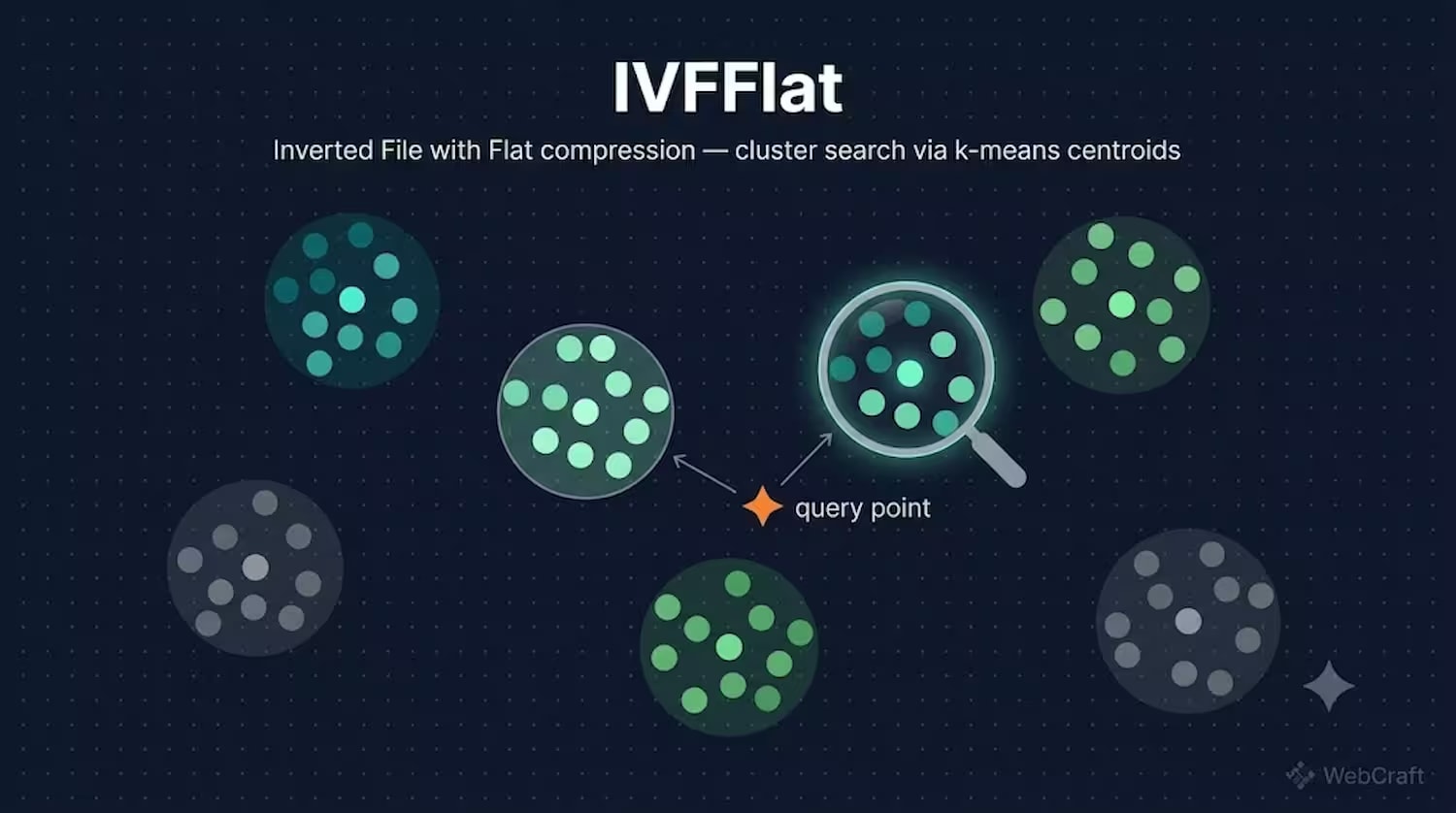
IVFFlat (Inverted File with Flat compression) takes a different approach: it divides the entire vector space into clusters (Voronoi cells) using k-means, each with its own centroid. During search, it first identifies the clusters closest to the query vector (the number is controlled by the probes parameter), and then the search is performed only within these clusters.

Analogy: imagine a library where books are not arranged alphabetically, but by thematic sections — fiction, history, cooking. Instead of looking through every book in the library (brute-force), you first go to the desired section (the closest centroid), and then search for the specific book only among those located there (search within the cluster). If a book happens to be in the "wrong" section, you simply won't find it, no matter how many sections you browse. This is the fundamental limitation of IVFFlat: search quality depends on how successfully k-means has distributed vectors into clusters.

A key practical rule for the number of clusters (lists) is sqrt(N) for N vectors (PE Collective, April 2026).

Example of index creation:

-- For 10,000 vectors: lists = sqrt(10000) ≈ 100
CREATE INDEX ON vector_store
USING ivfflat (embedding vector_cosine_ops)
WITH (lists = 100);

During the search phase, the probes parameter controls accuracy — how many of the closest clusters to check. The more probes, the higher the recall, but the slower the search (as more clusters need to be scanned):

SET ivfflat.probes = 10;

SELECT id, content
FROM vector_store
ORDER BY embedding <=> '[0.012, -0.034, ...]'
LIMIT 10;

By default, probes = 1 — only one closest cluster is checked. This is fast, but if the query vector happens to be close to the boundary between two clusters, a relevant result might lie in the "neighboring" cluster, which will not be checked. Increasing probes to 5-10 is a common trade-off between speed and accuracy.

IVFFlat builds faster and consumes less memory than HNSW — but has lower recall, especially on high-dimensional data or large datasets. Here it's worth remembering that the vector dimension itself (e.g., 1536 vs 3072) affects not only the quality of semantics but also how "fuzzy" the cluster boundaries become with k-means — we discussed the choice of embedding dimension in more detail in the article "1536 vs 3072: Comparing Embeddings for Document Search and RAG".

The most important nuance: IVFFlat requires the data to be already in the table BEFORE index creation — the algorithm needs to "learn" the cluster centers from the actual data distribution. HNSW does not have this limitation.

There's another practical aspect that's easy to underestimate: the quality of the vectors themselves that end up in clusters directly depends on how the text was chunked before indexing. Overly small chunks produce "noisy" embeddings that k-means struggles to group into clear clusters; overly large ones mix multiple topics into a single vector, which also blurs cluster boundaries. We discussed this in more detail in the article "Chunking Strategies in RAG 2026: How to Properly Chunk Data for Production".

HNSW vs IVFFlat: Comparison Table with Numbers

Sources for parameter values: Nerd Level Tech, May 2026; PE Collective, April 2026.

A separate independent study on real datasets (10-25 million vectors — SIFT, OpenAI, Cohere embeddings) shows that optimizations like half-precision (halfvec) provide practically the same search speed (QPS) with half the index size, and more aggressive binary quantization with re-ranking compresses the index 11-12 times — but with a noticeable drop in accuracy on some data types (study "Filter-Agnostic Vector Search on PostgreSQL", 2026). This is relevant if the HNSW index is close to the size of shared_buffers — a trade-off of "slightly lower accuracy for half the memory" is often justified at this stage, not earlier.

Summary from an independent Instaclustr benchmark: "Choose HNSW when accuracy and search speed are more important than index build time or memory usage. IVFFlat is a sensible choice for low-latency applications where build time or compactness are more important than the highest recall" (Instaclustr, February 2026).

IVFFlat Trap: Stale Centroids

This is the most common and costly mistake with pgvector — and it's easily reproducible in Spring AI projects precisely because of initialize-schema=true.

Scenario: A team creates an index CREATE INDEX ... USING ivfflat on the first application startup — when the vector_store table is still empty or has only a few test rows. The K-means centroids are calculated based on this unrepresentative data.

What happens technically: the k-means algorithm looks at the few vectors present at the time of index creation and partitions the entire future space into clusters around them. If at that moment the table contained, say, 5 test rows — the centroids "freeze" in a shape corresponding to these five points. When thousands of real documents are later loaded, they physically enter the vector space, but the logical structure of the clusters no longer matches the new data distribution. Some new vectors end up "far" from their nearest centroid simply because no centroid was actually calculated considering their existence.

The result is that all subsequent searches are performed against an index with "stale" centroids. Recall quietly degrades: a query that should find a relevant document doesn't find it because the document fell into an "unlucky" cluster that is never checked with the default probes = 1. The team spends months believing the problem lies with the quality of the embedding model or the chunking strategy, when the root cause is a single line in the database migration (Philip McClarence, Medium, April 2026).

The worst part about this error is its subtlety. There's no exception, no error in the logs, no application crash. The search simply works — but worse than it could. The RAG chat continues to respond, it just more often says "couldn't find relevant information" or pulls less accurate context. This is precisely the type of problem where the absence of an alarm is an alarm signal.

From my own experience: when we first encountered the bad SQL grammar error while Spring AI tried to automatically create an HNSW index on application startup (due to an outdated pgvector extension version on the hosting), the first thought is to simply switch index-type to ivfflat instead of none and move on. And this is exactly where it's easy to fall into the same trap unnoticed: initialize-schema=true in Spring AI means the index is created immediately on startup — and at that moment, the table is almost always empty. If we hadn't stopped then and figured out why HNSW failed with an error, but just "automatically" substituted IVFFlat as a replacement — we would have ended up with a working application with a subtly broken search, and would only find out when users started complaining that the chatbot "doesn't understand" simple questions.

Recommendation from the same source: "IVFFlat indexes do not belong in schema migrations. They belong in post-load scripts. HNSW is a safe default for applications up to 1M rows". This is not just a stylistic suggestion — it's a distinction by purpose: a schema migration describes the database structure, not its content, whereas IVFFlat is inherently tied to content.

Case 1: Blog with 800 Articles — Why We Don't Use Any Index

Our blog webscraft.org has ~800 articles (originals in Ukrainian + EN/DE/ES translations) and a RAG chat based on Spring AI + pgvector. The current state of the vector_store table:

SELECT COUNT(*) FROM vector_store;
-- 10852

Configuration in application.properties:

spring.ai.vectorstore.pgvector.initialize-schema=true
spring.ai.vectorstore.pgvector.distance-type=cosine_distance
spring.ai.vectorstore.pgvector.dimensions=${SPRING_AI_VECTORSTORE_PGVECTOR_DIMENSIONS:1536}
spring.ai.vectorstore.pgvector.index-type=none

Honest story: index-type=none was not an architectural decision from the start. On managed Postgres hosting, during the first deployment, Spring AI tried to automatically execute:

CREATE INDEX IF NOT EXISTS spring_ai_vector_index
ON public.vector_store USING HNSW (embedding vector_cosine_ops)

and failed with a bad SQL grammar error — the pgvector extension version on the hosting was outdated and did not support HNSW syntax (added only in pgvector 0.5.0, August 2023). The quick solution was index-type=none, and it remained in production — because further analysis showed: at 10,852 rows, it's not just "working," but is the optimal solution.

Why: the threshold where an ANN index truly starts to pay off is approximately 50,000 vectors (at smaller volumes, a brute-force scan takes milliseconds, while the overhead of building and maintaining HNSW/IVFFlat adds complexity without measurable benefit). With a growth rate of 3-4 articles per week, reaching this threshold is a matter of years, not months.

Case 2: Service with Tens of Thousands of Documents — Why IVFFlat is Appropriate There

Another project of ours, askyourdocs.org, is designed differently: it's a self-hosted service with the principle of single-tenant per deployment — each client gets their own fully isolated instance with a separate database (separate deployment on Railway, separate ENV variables). One client's data is not physically in the same table as another client's data. Architecturally, growth to tens of thousands of documents within one such database is expected — a scale where brute-force is no longer an option. Configuration:

spring.ai.vectorstore.pgvector.initialize-schema=true
spring.ai.vectorstore.pgvector.distance-type=cosine_distance
spring.ai.vectorstore.pgvector.dimensions=${PGVECTOR_DIMENSIONS:1536}
spring.ai.vectorstore.pgvector.index-type=${PGVECTOR_INDEX_TYPE:ivfflat}

IVFFlat is chosen here consciously: documents are loaded in batches (a client uploads a set of files once, then primarily only reads/searches), which matches the scenario "data loaded once, queried frequently" — precisely the case where IVFFlat is a sensible choice according to PE Collective's assessment (April 2026).

An important architectural nuance for this deployment model: since each client has its own separate database, the k-means centroids for IVFFlat are built exclusively on the documents of that specific client — without the "noise" from other people's data that would be a problem in a shared multi-tenant table filtered by userId. This removes a class of problems with filtered search, but adds another nuance: the moment a client uploads their first batch of documents is also the moment the database transitions from "empty" to "real" — and it's here that initialize-schema=true on the first deployment can easily create an IVFFlat index on an empty table, before any documents are loaded.

Practical conclusion for such an architecture: IVFFlat should be built or rebuilt after the initial loading of a representative volume of documents for a specific client (not immediately on deployment via initialize-schema=true), and periodically REINDEX as the client continues to load new documents — otherwise, the centroids will age exactly as described in the trap section above. For a self-hosted model, this means: the step "rebuild index after initial load" should be part of the new client onboarding process, not a one-time setup at the application level.

Practical Recommendation: How to Monitor the Transition Point

There's no need to guess when to switch to an index. On our blog, we've boiled it down to two simple metrics that we check quarterly — without any automation or dashboards, just calendar reminders.

-- 1. Size of the vector_store table
SELECT COUNT(*) FROM vector_store;

We run this query manually through PgAdmin in a minute. At the time of writing this article, we have 10,852 rows — and we are consciously in no hurry to change anything, as there is still a lot of time left until the approximate transition threshold at our growth rate (3-4 articles per week).

If you already have RAG query logging (we have a separate table for this with an admin panel — we described it in the section on query processing), the second signal is the search duration (durationMs) over time. An increase in this indicator is an earlier and more accurate indicator than the table size itself, as it also depends on server load. We pay attention to it not as an exact metric, but as a trend: if the average durationMs per week noticeably increases from week to week — this is a signal to look more closely, even if the absolute number of rows doesn't look threatening yet.

Frankly, the hardest part of this approach is not the check itself, but the discipline to do it regularly when everything is working fine. It's easy to postpone "until next quarter" and forget. That's why we chose the simplest possible query and the smallest possible number of metrics (only two) — we simply wouldn't maintain more complex monitoring on a permanent basis for a project of this scale.

Frequently Asked Questions (FAQ)

Can I just always use HNSW "just in case"?
You can, but on small datasets (up to ~30-50K rows), it doesn't provide a measurable speed benefit, while consuming memory and adding time to build/rebuild the index with every mass data reindexing.

What to do if the hosting has an old version of pgvector and HNSW is not supported?
Check the version: SELECT extversion FROM pg_extension WHERE extname = 'vector';. If the hosting allows — update the extension. If not, and the data volume is small — index-type=none is a perfectly working solution, not a temporary hack.

Is there anything better than HNSW for very large datasets?
Yes — DiskANN (via the pgvectorscale extension), which keeps a compact navigation structure in memory, and the vectors themselves — on disk, accessing them only for final candidate refinement. It's useful when the HNSW index exceeds the volume of shared_buffers (dbi-services, March 2026).

What are the easiest HNSW/IVFFlat mistakes to make?
I would highlight four that I've encountered myself or seen in other projects:

Mistake #1 — using HNSW on 50,000 documents.
I myself once thought that a "bigger and better" index couldn't hurt. In practice, at this volume, the additional memory and build time of HNSW provide no tangible speed advantage compared to simple index-type=none — you're just paying complexity for a benefit that isn't there at this scale yet.

Mistake #2 — creating IVFFlat before loading data.
This is the exact centroid trap I detailed above — and it's not a theoretical problem, I fell into this trap myself through initialize-schema=true in Spring AI. If the index is built on an empty or nearly empty table, it remains broken until you explicitly perform REINDEX after the actual data loading.

Mistake #3 — setting lists = 10 for a million vectors.
Here I would advise always keeping the sqrt(N) rule in mind: for a million vectors, this is approximately 1000 clusters, not 10. Too few clusters means that each of them contains a huge number of vectors, and searching within such a "giant cluster" is little different from brute-force on the entire table — you lose all the benefits of IVFFlat but pay for its maintenance complexity.

Mistake #4 — not running ANALYZE.
This mistake is the easiest to forget because it's not directly related to the index itself. After mass insertion or deletion of data, the Postgres planner's statistics become outdated, and it may simply not choose your index during query execution, even if the index is perfectly built. I've made it a habit to run ANALYZE vector_store; immediately after any mass reindexing — it takes seconds, but saves you from the situation "the index exists, but Postgres doesn't use it."

Conclusions

Summary Cheat Sheet: HNSW vs IVFFlat in One Table

To summarize all the discussion in one sentence: HNSW trades insertion speed and memory for search speed and accuracy, IVFFlat does the opposite. Which side of this trade-off is more important depends solely on your workload pattern, not on which index is "better" in an abstract sense.

• An index (HNSW or IVFFlat) is an optimization for scale, not a mandatory component of any pgvector project.
• At volumes up to ~30-50 thousand vectors, brute-force search (index-type=none) is usually faster than the overhead of index maintenance.
• HNSW is a safer default for unpredictable data changes (new content added gradually): it doesn't depend on insertion order, doesn't require REINDEX.
• IVFFlat is appropriate when data is loaded in large batches once and queried frequently — but requires building the index *after* loading a representative amount of data and periodic REINDEX as it grows.
• The most costly mistake is creating an IVFFlat index on an empty table through automatic schema initialization. Recall degrades silently, and it's easy to confuse with embedding model issues.